Note
This page was generated from a Jupyter notebook. You can download the notebook from the notebooks/ directory in the repository.
Hyperspectral Images Manipulation
Author: Riccardo Finotello riccardo.finotello@cea.fr
This notebook explores the HSIMars class to manipulate and display the hyperspectral images (HSI) of Mars exploration.
[1]:
%load_ext autoreload
%autoreload 2
[2]:
from hsimars import HSIMars
First Steps
We first need to instantiate the HSIMars class:
[3]:
hsi = HSIMars(
    hdr_path="../data/HC_frt0000580c_07_if164j_ter3.hdr",
    annotations="../data/HC_ground_truth.mat",
)
We then proceed with the extraction of the HSI:
[4]:
img = hsi.get_img()
type(img)
[4]:
hsimars.hsi.HSIMarsImageData
The object is a namedtuple containing several attributes, which can be accessed using the usual Python interface img.<attr>:
hsi: the HSI data,wavelength: the list of wavelengths (units: nm),shape: the shape of the image,height: the height of the image,width: the width of the image,channels: the number of channels in the image,dtype: the data type of the HSI.
[5]:
print("img.hsi -->", type(img.hsi))
print("img.wavelength -->", type(img.wavelength))
print("img.shape -->", type(img.shape))
print("img.height -->", type(img.height))
print("img.width -->", type(img.width))
print("img.channels -->", type(img.channels))
print("img.dtype -->", type(img.dtype))
img.hsi --> <class 'numpy.ndarray'>
img.wavelength --> <class 'numpy.ndarray'>
img.shape --> <class 'tuple'>
img.height --> <class 'int'>
img.width --> <class 'int'>
img.channels --> <class 'int'>
img.dtype --> <class 'str'>
We can also recover the annotations using the same principle:
[6]:
ann = hsi.get_annotations()
type(ann)
[6]:
hsimars.hsi.HSIMarsAnnotationData
The output is another namedtuple, containing the following attributes:
labels: the annotation data,shape: the shape of the image,height: the height of the image,width: the width of the image,dtype: the data type of the annotation.
[7]:
print("ann.labels -->", type(ann.labels))
print("ann.shape -->", type(ann.shape))
print("ann.height -->", type(ann.height))
print("ann.width -->", type(ann.width))
print("ann.dtype -->", type(ann.dtype))
ann.labels --> <class 'numpy.ndarray'>
ann.shape --> <class 'tuple'>
ann.height --> <class 'int'>
ann.width --> <class 'int'>
ann.dtype --> <class 'str'>
If you prefer, you can also call both of these outputs at the same time:
[8]:
img, ann = hsi.data()
type(img), type(ann)
[8]:
(hsimars.hsi.HSIMarsImageData, hsimars.hsi.HSIMarsAnnotationData)
Visualisation
You can also visualise the annotations and the image (in fake colours) using opencv (a new window will open, close it with “q”):
[9]:
hsi.display_hsi()
You can visualise the annotations (close the new window with “q”):
[10]:
hsi.display_annotations()
Or you can display all of the information at once (close again with “q”):
[11]:
hsi.display()
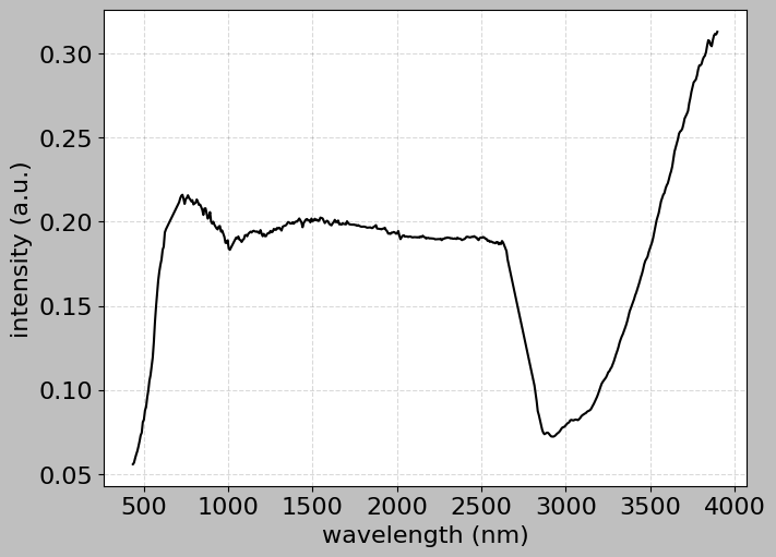
We can also plot a particular spectrum:
[12]:
hsi.plot_spectra((128, 145))
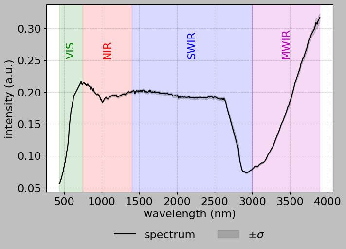
[13]:
hsi.plot_spectra([[128, 145], [129, 146], [128, 146], [129, 145]], bands=True)
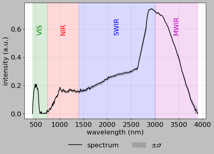
[14]:
hsi.plot_spectra(
    [[128, 145], [129, 146], [128, 146], [129, 145]],
    convex_hull=True,
    bands=True,
)
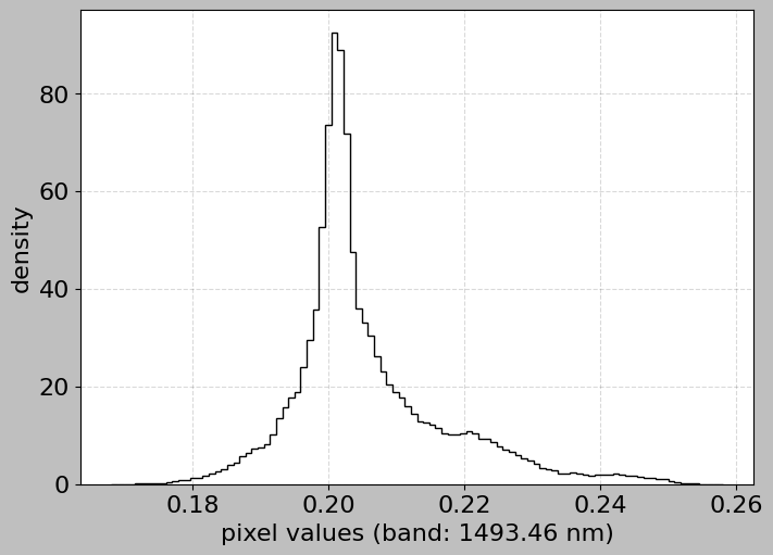
Or even the histogram of a particular band:
[15]:
hsi.plot_histogram(band=146)

[16]:
hsi.plot_histogram(band=1493.0)
Working with Label Names
The annotation data includes a label_names dictionary that maps numerical labels to human-readable mineral names:
[17]:
# Get annotation data
img_data, ann_data = hsi.data()

# Display the label names mapping
print("Available mineral classes:")
for label_id, mineral_name in sorted(ann_data.label_names.items()):
    print(f"  {label_id}: {mineral_name}")
Available mineral classes:
  1: Analcime
  2: Plagioclase
  3: Prehnite
  4: High-Ca Pyroxene
  5: Serpentine
  6: Margarite
[18]:
# Count pixels for each mineral class
import numpy as np

unique_labels = np.unique(ann_data.labels)
unique_labels = unique_labels[unique_labels > 0]  # Exclude background

print("\nClass distribution:")
for label_id in sorted(unique_labels):
    count = np.sum(ann_data.labels == label_id)
    mineral_name = ann_data.label_names.get(
        label_id, f"Unknown (ID: {label_id})"
    )
    percentage = (count / ann_data.labels.size) * 100
    print(f"  {mineral_name:25s} - {count:6d} pixels ({percentage:5.2f}%)")
Class distribution:
  Analcime                  -    940 pixels ( 0.37%)
  Plagioclase               -   1472 pixels ( 0.59%)
  Prehnite                  -   1560 pixels ( 0.62%)
  High-Ca Pyroxene          -   6963 pixels ( 2.78%)
  Serpentine                -   8697 pixels ( 3.47%)
  Margarite                 -    458 pixels ( 0.18%)